Google BigQuery ML (BQML) is a powerful tool that allows data scientists and analysts to build and deploy machine learning models directly within Google BigQuery. By integrating machine learning into BigQuery, BQML eliminates the need to move data between various systems or platforms, enabling you to utilise data science to extract data-driven insights efficiently. This simplifies the workflow and reduces the time to develop and operationalise ML models.
You can build and train models using SQL queries, allowing for easy integration with existing data pipelines. BQML supports a variety of model types, including linear and logistic regression, ARIMA models, and more, enabling you to tackle a wide range of predictive analytics tasks efficiently.
Using BigQuery ML for data analysis is made significantly easier due to its seamless integration with Looker Studio (previously known as a data studio), Google’s powerful data visualisation and business intelligence tool. This connection allows users to directly visualise, explore, and share insights from their BigQuery ML models without the need for complex data transfers or additional processing. Looker Studio provides an intuitive, drag-and-drop interface for creating rich, interactive dashboards that can display real-time results from BQML models.
Additionally, you can use BigQuery ML to provide some elementary insights into media effectiveness by leveraging its machine learning capabilities to analyse and optimise media strategies. It enables quick predictive modelling to forecast campaign impacts, audience segmentation for tailored targeting, and multi-touch attribution to understand the contribution of each media touchpoint. Its seamless integration with tools like Looker Studio and Google Analytics ensures comprehensive analysis and easy implementation of insights.
Key functions
Google BQML breaks the task of building and operationalising ML models into 3 steps, each associated with its own function. The typical workflow in BQML begins with the creation of the model, it is here that parameter estimation takes place. This is then followed by an evaluation of the model, in which precision and accuracy are analysed. Lastly, the model is then used to perform prediction.
The “CREATE MODEL” statement
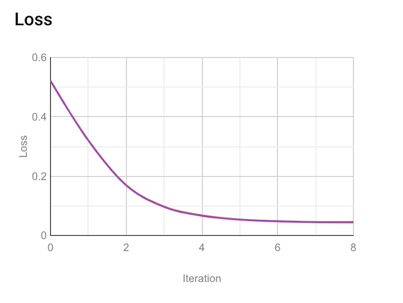
The first step when developing any ML model is to build it, which involves parameter estimation. During the creation of the model, BQML automatically splits the data into training and testing subsets, enabling you to assess the predictive accuracy of your given model. Parameter estimation is performed in BQML by minimising the loss statistic, a metric describing how well the model predicts the test dataset. If predictions are close to the unseen data then the loss should be close to 0.
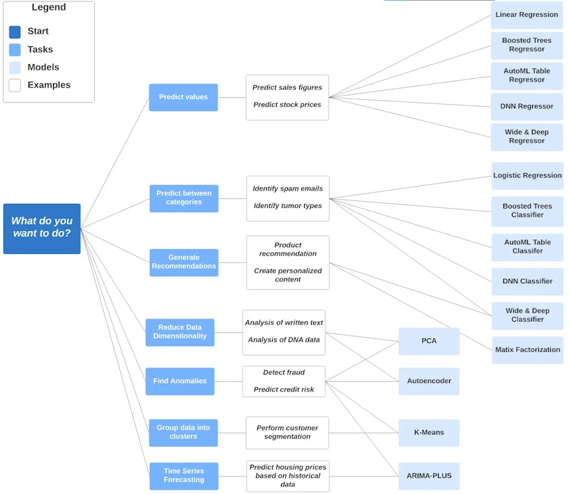
Additionally, the “CREATE MODEL” statement is where you specify the type of model you wish to build. The model you build should be relevant to the objective in mind. BQML has provided this guide to help with selecting the right model.
The “ML.EVALUATE” function
The second step in the ML workflow is to evaluate the performance of the model, which is done in BQML using the “ML.EVALUATE” function. This function evaluates the predicted values generated by the model against the actual data for both the training and the testing datasets. Outputs may vary depending on the type of model you build, the following metrics are standard output when working with a logistic regression model, in which binary classification is the objective in mind:
- precision: a metric for classification models which identifies the frequency with which a model was correct when predicting the positive class.
- recall: a metric for classification models that tells you how many positive labels, out of all the possible positive labels, you correctly identified.
- accuracy: a metric for classification models that tells you the fraction of predictions that a classification model got right.
- f1_score: measures the overall accuracy of the model. An f1 score lies between 0 and 1, 1 indicating optimal accuracy.
- log_loss: This is the measure of how far the model’s predictions are from the correct labels. The log is used due to the nature of logistic regression.
- roc_auc: refers to the area under the ROC curve, which is the probability that a classifier is more confident that a randomly chosen positive example is actually positive than that a randomly chosen negative example is positive.
The “ML.PREDICT” function
The “ML.PREDICT” function allows you to forecast from the model, however, care must be taken with forecasting as ML models tend to lose predictive accuracy the further away we extrapolate from the known data set. By applying this function, you can easily predict outcomes based on new input data directly within BigQuery.
Time series forecasting
Time series forecasting is crucial in digital marketing as it enables you to predict future trends and customer behaviours based on historical data, allowing for more informed decision-making and strategic media planning. By leveraging time series forecasting, you can anticipate peak periods, optimise campaign timing, and allocate budgets more effectively to maximise ROAS.
Integrating time series forecasting with Marketing Mix Modeling (MMM) further enhances its value, as MMM helps quantify the impact of various marketing channels and activities on sales and other key performance indicators. This combination allows you to not only forecast future outcomes but also understand the drivers behind these predictions, enabling a more holistic and data-driven approach to campaign optimization and resource allocation.
Introduction and objectives
In this example, we’ll create an ARIMA time series model to perform single time-series forecasting using the google_analytics_sample.ga_sessions sample table. The ga_sessions table contains information about a slice of session data collected by Google Analytics 360 and sent to BigQuery. We’ve extracted the daily number of website visits from 2016-08-01 to 2017-08-01.
The objective is to forecast the number of website visits for August 2017.
The first step in creating any form of ML model is to understand the data you’re modelling. The visual below shows the data we’ll be modelling.
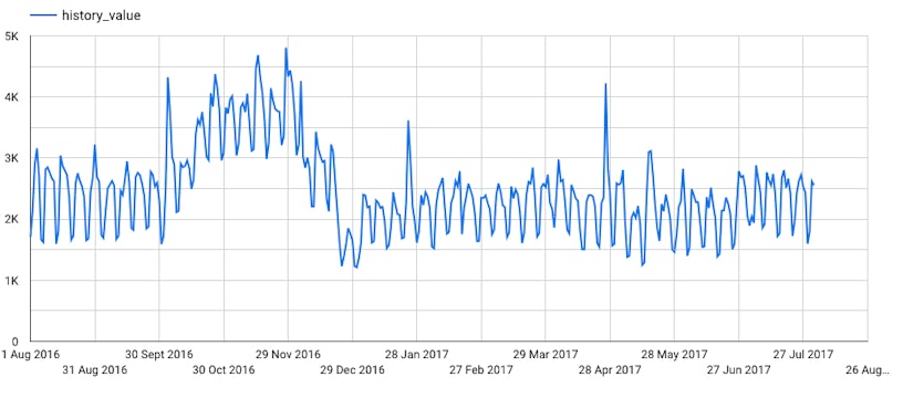
At first glance, this time series exhibits an increasing trend until ~November 2016. This trend then starts to decrease until December 2016, telling us that we have a non-constant mean. This indicates that perhaps taking the first difference might eliminate the trends present in this data.
Furthermore, the variance of this time series does appear to be somewhat constant over time, with very few peaks and troughs standing out. This indicates no need for a transform to eliminate fluctuations in variance.
Model creation and evaluation
Now we’ve familiarised ourselves with the data and identified the type of model we require, the next step is to run the “CREATE model” statement. As we’re going to use an ARIMA model we’ll need to specify “model_type = ‘ARIMA_PLUS’”. By default, the algorithm fits dozens of candidate models and automatically tunes the hyperparameters. BQML chooses the model with the lowest Akaike information criterion (AIC).
After creating your model, the next step is to evaluate its performance. To do this we simply run the “ML.EVALUATE” function and observe our outputs. Upon running this, you should find the outputs of up to 42 candidate models, notice that the optimal model is the one with the lowest AIC which is always on row 1. The relevant outputs for row 1 are as follows:
| p | d | q | has_drift | AIC | variance |
|---|---|---|---|---|---|
| 2 | 1 | 3 | true | 4885.81 | 36334 |
This tells us we’re forecasting from an ARIMA(2,1,3) with an intercept term.
For more information on the nature of our model, we can run the “ML.ARIMA_COEFFICIENTS” function to extract the values of the coefficients of our model as tabulated below.
| ma1 | ma2 | ar1 | ar2 | ar3 | intercept |
|---|---|---|---|---|---|
| -0.1498 | -0.6834 | -0.2523 | -0.6894 | -0.6484 | 2.6125 |
Overall, our model has 2 non-seasonal moving average components, 3 non-seasonal autoregressive components and has non-seasonal difference of order 1. This model is optimal, suggesting that there is no need for seasonal components for forecasting.
It is important to point out here that when building an ML model, model diagnostics should be a part of your workflow! Fortunately for us, the “ML.EXPLAIN.FORECAST” function allows you to extract your residuals for conducting residual analysis.
Forecasting
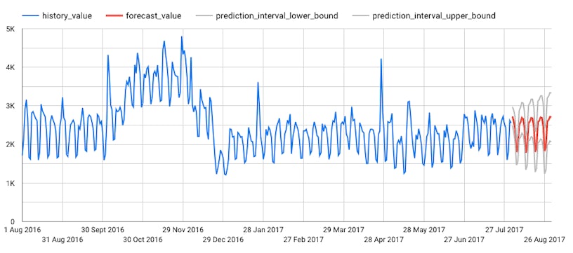
Now we have evaluated our model and are familiar with its various components, then the next step is to forecast the number of website visits for August 2017. To do this we make use of the “ML.FORECAST” function, which produces both future time series values and prediction intervals. The following forecasts were produced.
Now that we have our daily forecasts, we may wish to summarise them for the whole of August. The table below shows the forecasted total number of website visits, along with the associated upper and lower bounds.
| Total mean forecast | Total upper forecast | Total lower forecast |
|---|---|---|
| ~72,029 | ~57,667 | ~86,392 |
On average we expect to see 72,029 website visits during August 2017. We should expect to see at least 57,667 and at most 86,392.
Logic regression
Logistic regression is a particularly valuable tool to have in digital marketing as it provides a robust method for predicting binary outcomes, such as customer conversion or click-through rates, based on various predictor variables like user behaviour, demographic information, and past interactions. Through logistic regression, you can identify the key factors that influence customer decisions and tailor their strategies to target high-probability converters more effectively.
Additionally, logistic regression can be seamlessly integrated with RFM (Recency, Frequency, Monetary) modelling to predict customer behaviours such as purchase likelihood, enabling you to target and engage the most valuable customer segments more effectively.
Introduction and objectives
In this example we create a logistic regression model using BigQuery ML. We’ll use the Google Analytics sample dataset to create a model that predicts whether a website visitor will make a transaction. If the number of transactions within the session is “NULL”, we assign this to a value of 0. Otherwise, it is set to 1. These values represent the possible outcomes.
Given we only have existing data up to 30th June 2017, the objective of this model is to predict the number of website visitors that will make a transaction throughout July 2017.
To model the probability that a website visitor will complete a transaction, the following predictor variables have been used:
- The operating system of the visitor’s device.
- The device they used to visit the website.
- The country from which the session originated.
- The number of page views within that session.
Model creation and evaluation
Now we have all our variables defined and have identified the type of model we require, the next step is to run the “CREATE model” statement. We’re running the model using daily data from 2016-08-01 to 2017-06-30.
After creating your model the next step is to evaluate its performance. To do this we simply run the “ML.EVALUATE” function and observe our outputs. The outputs of doing so are tabulated below:
| precision | recall | accuracy | f1_score | log_loss | roc_auc |
|---|---|---|---|---|---|
| 0.4685 | 0.1108 | 0.9853 | 0.1792 | 0.0462 | 0.9817 |
As we can see, the model metrics here are quite low and significantly far away from the maximums, indicating we have plenty of room for improvement and should reconsider. For a “good” model, we should expect most of these metrics (apart from the log_loss) to be close to 1. For the purposes of this blog, we’re going to continue with this model and produce some predictions.
Prediction
Using the “ML.PREDICT” function, we’ve predicted the number of transactions made by website visitors from the USA for July 2017.
| Country | Number of Transactions |
|---|---|
| USA | 220 |
Therefore the number of transactions made by website visitors from the USA for July 2017 is predicted to be approximately 220.
Conclusion
In conclusion, Google BigQuery ML offers a robust easy-to-use platform for integrating machine learning directly within your data warehouse environment. By leveraging the CREATE MODEL, ML.EVALUATE, and ML.PREDICT functions, you can seamlessly build, evaluate, and deploy models using standard SQL queries. The example of ARIMA forecasting demonstrates the powerful capabilities of BQML for time series analysis, allowing for accurate forecasts and insightful analytics.
Whether you are looking to perform classification, regression, or time series forecasting, BigQuery ML provides the tools necessary to streamline your machine learning workflows, making advanced analytics accessible and efficient.