In digital marketing, A/B testing is a technique for comparing two versions of a variable, such as a landing page layout or ad creative, to determine which version performs best with the target audience. The audience is randomly divided into two groups: one group is exposed to version A (the control), and the other to version B (the variant). Key performance indicators (KPI’s), such as conversions, are then tracked to evaluate each version’s performance.
However, simply observing which version has a higher number of conversions doesn’t guarantee that the observed difference is due to the change itself. Random fluctuations or sampling variability can cause apparent differences that may not be meaningful. So, how can we be confident that any observed difference reflects a true effect rather than just chance? This is where statistics and data science come into play to help quantify the uncertainty around our results and provide a rigorous basis for decision-making.
- The Bayesian approach to A/B testing
- Frequentist approach
- Bayesian approach
- Bayesian A/B Testing Implementation in CRO
- Define your hypothesis
- Collect and Interpret your data
- Choose your prior conversion rates
- Calculate the posterior conversion rates
- Calculate the probability of superiority
- Calculate the conversion rate uplift
- Interpret your results
- Take action
The Bayesian approach to A/B testing
Statistics provides a framework for quantifying uncertainty, allowing us to make informed decisions even in the presence of incomplete information. This uncertainty is quantified through probability, giving us a way to understand the likelihood of different outcomes based on available data.
In Bayesian statistics, probability is viewed as a measure of certainty in a particular outcome and prior knowledge or beliefs are incorporated into the analysis. In Bayesian A/B testing, the process begins with a prior belief (or distribution) about the effectiveness of each version (A and B), which might be informed by historical data, expert opinion, or previous experiments. As new data from the A/B test is collected, the Bayesian approach updates this prior belief using Bayes’ theorem, resulting in a posterior probability distribution that reflects both the prior knowledge and the new evidence. This approach is particularly useful because it allows you to continuously refine your estimates as more data becomes available, leading to probability-based confidence in which version is likely to perform better.
In A/B testing, both Bayesian and Frequentist approaches serve distinct purposes:
Frequentist approach
This approach is often valued for its objectivity and clear decision criteria, such as achieving statistical significance at a specific p-value threshold. However, it requires a fixed sample size and doesn’t directly tell us the probability that one version is better than the other. It only indicates whether the observed difference is likely due to chance.
Bayesian approach
This approach, by contrast, provides a direct probability that one version is better than the other, allowing for a more flexible interpretation of the results and enabling dynamic decision-making as data accumulates. This flexibility is particularly advantageous in digital marketing, where strategies often need to be adjusted in real-time based on rapidly changing user behaviours and market conditions.
Bayesian A/B Testing Implementation in CRO
The remainder of this blog will walk you through how to implement your own Bayesian A/B test. While there are many A/B testing tools available that can quickly provide probabilities, uplift estimates, and other key metrics, understanding the internal workings behind these tools is crucial. Knowing how concepts like posterior probabilities, credible intervals, and Bayesian inference work enables you to interpret results more effectively and make smarter decisions. It also helps you recognize the limitations of automated tools, ensuring that your strategies are based on sound analysis rather than blind trust in numbers.
Define your hypothesis
The first step in any A/B test is to define your hypothesis, this is an experiment after all.
In the context of conversion rate optimisation (CRO), the null hypothesis (H0) and the alternative hypothesis (H₁) are defined as follows:
- Null Hypothesis (H₀): There is no difference in the performance between version A (the control) and version B (the variant). Any observed difference in conversion rates is purely due to random chance. Mathematically, this is expressed as:
H0: CRA = CRB
- Alternative Hypothesis (H₁): There is a statistically significant difference in performance between version A and version B. This means that any observed difference is likely due to the actual effect of the changes made in version B, rather than random chance. This can be one-sided (suggesting that one version performs better than the other) or two-sided (suggesting that the two versions perform differently, without specifying which is better). A two-sided alternative hypothesis can be mathematically expressed as:
H1: CRA ≠ CRB
Collect and Interpret your data
Randomly assign users from the target audience to one of groups A or B and collect the relevant conversion data. Your dataset should look something like the following:
| Sample Size | Number of Conversions | |
| Group A | 2100 | 58 |
| Group B | 2155 | 79 |
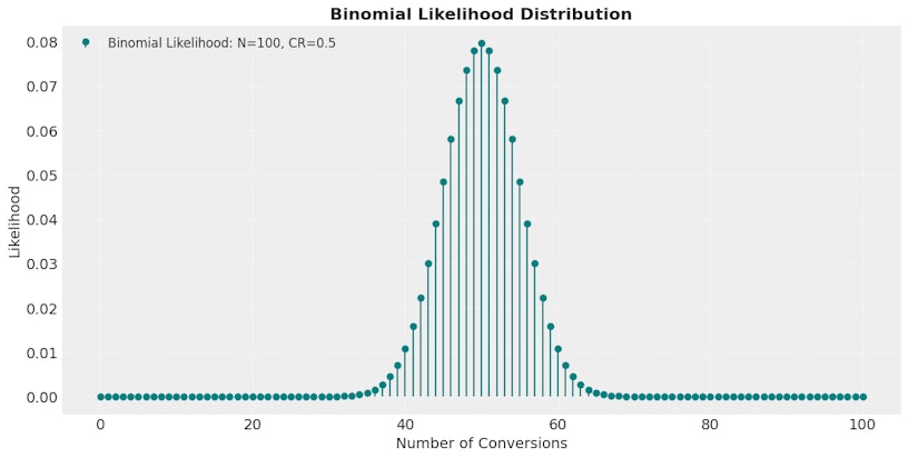
To interpret our data, we need to think about the underlying likelihood of our data.
We know that a random user from group A will convert with an unknown conversion rate CRA. As this outcome is binary (convert = 1 or not convert = 0), the event that a random user (X1A) in group A will convert, given the conversion rate CRA, can be described using a Bernoulli distribution:
X1A | CRA ~ Bernoulli(CRA)
Given we have NA users in group A, the likelihood of our data for group A is given by the sum of NA Bernoulli trials.
(X1A + X2A + … + XNA | CRA)
Which follows the Binomial distribution:
(X1A + X2A + … + XNA | CRA) ~ Binomial(NA,CRA)
Through similar analysis, the likelihood of our data for group B is given by:
(X1B + X2B + … + XNB | CRB) ~ Binomial(NB,CRB)
Now we’ve collected our data and determined the likelihood distributions of both groups follow a binomial distribution, the next step is to choose your prior.
Choose your prior conversion rates
A non-informative prior is used when we have little to no prior knowledge about the likely outcomes. It ensures the data will primarily drive the results rather than any preconceived assumptions. An informative prior, on the other hand, incorporates existing knowledge or beliefs about the expected outcome based on past experiments, domain expertise, or historical data. Informative priors can risk introducing unwanted bias if the prior is inaccurate.
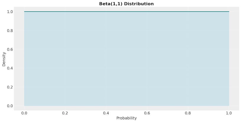
In the case where we have very little (if any) knowledge of expected outcomes, a commonly used non-informative prior is a Beta(1,1) distribution, a special case of the Beta distribution.
CRA ~ Beta(1,1)
This prior assumes the true conversion rate exists anywhere between 0 and 1, with equal probability.
Calculate the posterior conversion rates
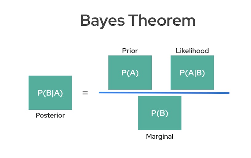
In Bayesian statistics, calculating the posterior distribution is essential to updating beliefs about a hypothesis given observed data, and this is achieved using Bayes’ theorem. Here, Bayes’ theorem combines prior knowledge (the prior distribution) with new data (through the likelihood) to compute the posterior distribution, which represents an updated probability of the hypothesis.
For the full computation of the posterior, we need the prior, the likelihood, and the marginal probability of the observed data. The marginal probability (also called the evidence) is typically challenging to calculate directly since it involves integrating all possible values of the parameter, which can be computationally expensive or infeasible in complex models such as Marketing Mix Models (MMM). Therefore, in many cases, we rely on advanced sampling techniques, such as Markov Chain Monte Carlo (MCMC), to approximate the posterior.
However, in Bayesian A/B testing, if we use a non-informative prior, such as a Beta(1,1) distribution, our computation simplifies significantly. This prior (and any Beta prior) is conjugate to the binomial likelihood, meaning that when combined with binomial data, it produces a posterior that is also in the Beta distribution family. Conjugate priors are particularly useful in Bayesian analysis because they allow for an exact analytical solution of the posterior without the need for sampling methods.
By choosing a Beta prior with parameters that are either non-informative or reflective of prior knowledge, we can obtain an updated Beta posterior that directly incorporates our A/B testing results, making the Bayesian analysis more straightforward and computationally efficient.
After working through the Mathematics, we obtain the following posterior distribution for CRA:
(CRA | X1A + X2A + … + XNA) ~ Beta(ΣxA+1, NA–ΣxA+1)
Where
ΣxA is the total number of observed conversions in group A
Through similar analysis, the posterior distribution for CRB is given by:
(CRB | X1B + X2B + … + XNB) ~ Beta(ΣxB+1, NB–ΣxB+1)
Where
ΣxB is the total number of observed conversions in group B
Calculate the probability of superiority
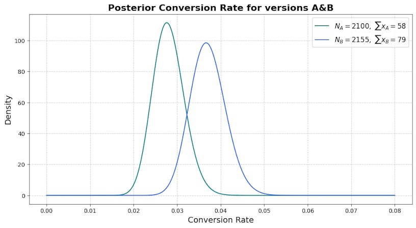
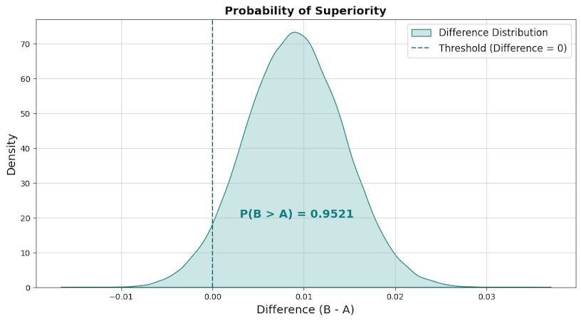
The probability of superiority quantifies the likelihood that one group (B) performs better than another (A). It is calculated by taking the difference between the posterior distributions of both versions and then determining the proportion of the resulting distribution that is greater than zero. This area under the density curve where the difference is positive represents the confidence that variant B is superior to control A.
For the visual below, the probability superiority is 95.2%.
Calculate the conversion rate uplift
The relative conversion rate uplift is given by the following:
CRB – CRA / CRA
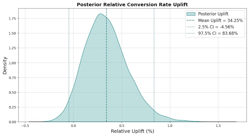
As we have posterior distributions for both CRA and CRB, we can now estimate the posterior relative conversion rate uplift. This is highly beneficial because the posterior provides Highest Density Intervals (HDIs) for the relative conversion rate uplift, offering a clear range within which the true uplift is most likely to fall. Unlike traditional methods that give a binary “significant or not” result, HDIs enable you to quantify uncertainty and understand the potential variability in uplift.
Interpret your results
The probability of superiority gives you the probability that one version is better than the other. In this case, variant B has a 95.2% probability of being superior to control A, meaning we have evidence to reject the null hypothesis and can be confident that version B is likely the better choice.
The posterior conversion rates can provide valuable insights too. You can use them to see the range of possible true conversion rates for each version. This range reflects uncertainty, so a wider interval means your data might not provide a clear answer, while a narrow interval boosts confidence. In this case, both distributions appear to have similar dispersion, but variant B is slightly wider. Although both are very similar in terms of uncertainty, we’re slightly less confident in the true conversion rate of variant B than control A.
Finally, the posterior conversion rate uplift shows how much better one version might perform, along with credible intervals that capture its uncertainty. In this case, the mean conversion rate uplift is 34.3%, meaning we estimate variant B will generate 34.3% more conversions on average than variant A. By analysing the credible interval, we can infer that variant B will generate between -4.56% and 83.68% more conversions with variant A with 95% probability. As this interval is very wide, we must take extreme caution when implementing variant B as standard.
When interpreting the results of your Bayesian A/B test, focus on the story your data is telling. Instead of just focusing on the average values, pay attention to credible intervals – they help you weigh the potential benefits of a change against the risks of uncertainty. By understanding both the insights and limitations of your results, you’ll make smarter, more confident decisions for your business.
Take action
With the results of your Bayesian A/B test in hand, it’s time to take action. The analysis shows that variant B has a 95.2% probability of being superior to control A, with an estimated average uplift of 34.3% in conversion rate. This strong evidence suggests implementing variant B as the new standard is a smart choice. Use the insights from the credible intervals (-4.56% to 83.68%) to set realistic expectations for performance improvements, account for the potential risks and plan your strategy accordingly.
Beyond simply adopting variant B, leverage what you’ve learned to iterate further by identifying the elements of variant B that drove the uplift and test additional refinements. Bayesian A/B testing isn’t just about finding “winners”, it’s about continuously learning and improving to drive sustainable growth for your business.