Every time I hear someone say “VLOOKUP”, I cringe. While many people have heard of the function, it seems that only a few people use it and even fewer use it correctly. What hurts me the most is that there’s a much better alternative that virtually no one uses: INDEX MATCH. In this post, I’m going to explain how to use this powerful tool for PPC campaigns and why you should probably never, ever, ever use VLOOKUP ever again.
Why VLOOKUP is terrible
There are a multitude of reasons not to use VLOOKUP.
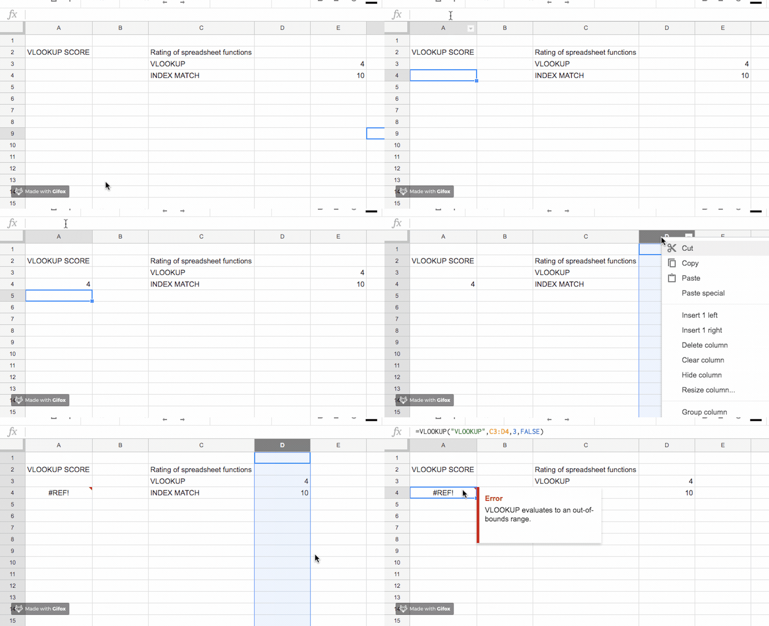
- You have to count the columns. This doesn’t sound like much of a big deal, but last week I was sent a spreadsheet of client data with 54 columns. To use VLOOKUP, I’d have had to count all of the columns up until the one that I wanted. The worst part is that if someone ever changed that table around (even so much as removing or moving one column) every single one of my VLOOKUP functions would break. Personally, I’d rather spend more time optimising campaigns than debugging spreadsheet formulas and I’m sure our clients would prefer that too.
- You can only look up values in the leftmost column of the table. That’s right, if what you’re looking for isn’t in the very first column, VLOOKUP can’t help you. Rearranging tables and duplicating columns to find a value might seem like an adequate solution, until you need to look something else up and you realise that you’ve snookered yourself.
- VLOOKUP doesn’t always give you the result you’re looking for. Admittedly, this is usually down to user error, but unless your data is sorted and you tell VLOOKUP that it’s sorted, it will look up the wrong value more often than not. If VLOOKUP doesn’t give you a (useless) error, it’ll give you what it considers “the nearest match” instead. In PPC, “the nearest match” could be a very expensive mistake.
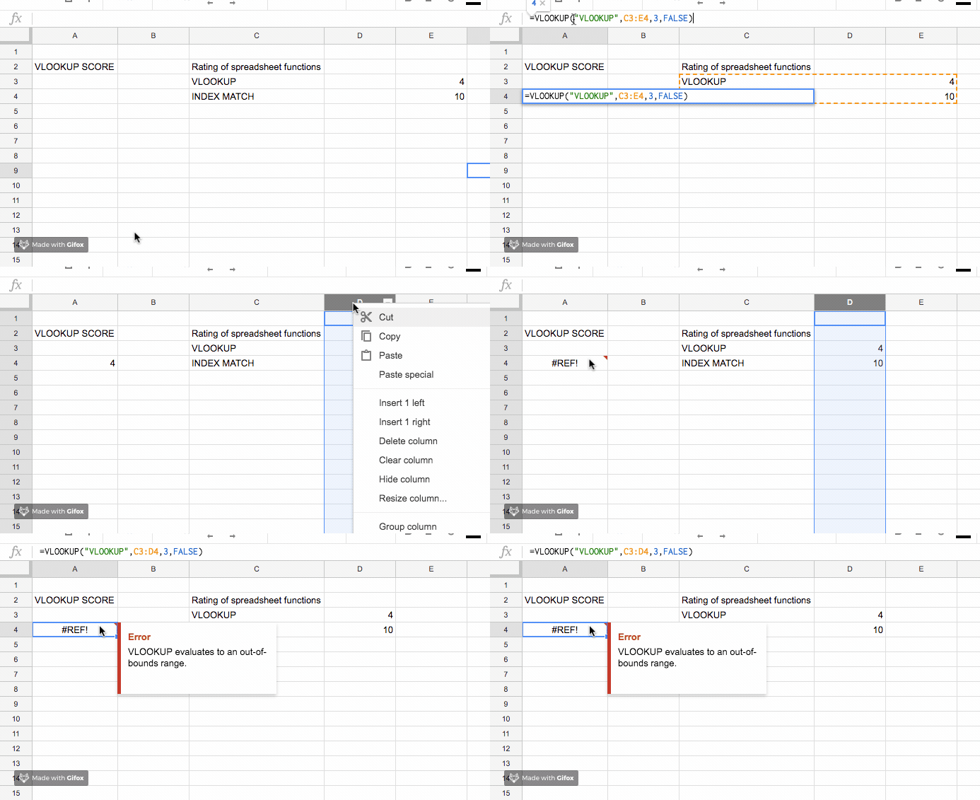

Wouldn’t you prefer to get the right result every time?
With INDEX MATCH:
- you can have dynamic column references (which means fewer errors)
- you can add as many or as few columns as you like without breaking everything
- your look up value can be in any column (or in any row)
If that wasn’t good enough, you can also use INDEX MATCH in both Google Sheets and Excel.
In short, INDEX MATCH is better than VLOOKUP in pretty much every single concievable way.

INDEX MATCH looks really intimidating at first. However, by the time you’ve got to the end of this post, you’ll feel like a spreadsheet ninja.
Introducing INDEX MATCH
Rather than attempting to search for a value which may or may not be in the range you’ve specified, INDEX MATCH allows you to turn the whole range into a grid and select exactly the cell that you’re looking for – every time. Technically speaking, INDEX MATCH isn’t a spreadsheet function, it’s two: INDEX and MATCH. Let me break them both down before explaining why they’re so much more powerful together and how to use them for PPC.
INDEX
INDEX returns the content of a cell which has been specified by a row or column index.
Remember the game Battleships where you had to guess where your opponent’s ships were by giving coordinates? This is pretty much the same thing, except instead of using letters, you use numbers.
The syntax is relatively simple when you know what it means:
INDEX(reference, row, column)
The reference is the range you want to look up, the row is the row number your target cell is in and the column is the column number your target cell is in. Super simple.
Let me give you an example to make it even clearer. Let’s say you’d been sent the following spreadsheet from (imaginary) client Smelly Socks – a retailer of fragranced footwear.

By entering the function =INDEX(A1:C3, 2, 3) into an empty cell, you’ll be presented with the value in C2.

Why C2? Because it’s the second row and third column of the range.
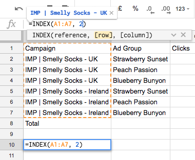
You can even use it with just columns (without rows) or just rows (without columns). For example, =INDEX(A1:A7, 2) would give you the result of whatever is in A2 because it’s the second row of the column.
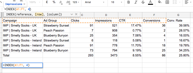
For rows, the second value specifies the row number, not the column number. That means that =INDEX(A1:F1, 4) will give you whatever is in D1 because that’s the fourth column.
Both row and column are optional if you don’t need them, but most of the time you’ll need both.
Select the whole table as the range and you will have free reign to navigate your way around every cell co-ordinates style.

Now that’s all well and good, except with INDEX, you need to know the co-ordinates to actually put it into the function. That doesn’t make it much better than VLOOKUP. However, that’s where MATCH comes in.
MATCH
MATCH is one of the most underrated functions in the whole history of spreadsheets. You know that counting you used to do to work out which column you wanted for VLOOKUP? No need – MATCH does it for you. It’s super clever. Rather than counting the number of columns or rows, it looks for an actual value in the column or row and tells you its location.
Confused? First, let me give you the syntax and then I’ll explain with an example.
The function is used as follows:
=MATCH(search_key, range, [search_type])
This looks really complicated. Bear with. All shall become clear.
- search_key is just the thing you’re searching for, usually a value in a header of some sort, e.g. “Clicks”, “Impressions”, “CTR” etc.
- range is just the range you want it to look for the value in. This has to be one-dimensional, e.g. it has to be a range containing either just one row or just one column. A straight line, basically. Something like A4:D4 or D4:D17 is fine, something like A4:D17 is not.
- [search type], which is optional, allows you to select which type of search you want it to do. Most of the time, you’ll want to set this to “0” which is exact match. (If your data is sorted, there are two other options you can use – like finding either the largest value less than or the smallest value greater than your lookup value. For more information about those, see MATCH – Doc editors Help for Google Sheets or MATCH function – Office Support if you’re using Excel. Both work in the same way.)
Lost? Stay with me, it’s example time. Here’s the data from Smelly Socks from before.

Let’s say I want to find the click-through rate which is in column E. Since there are only a few columns, I could count this and work out which column it’s in, but since I want to be efficient and make my spreadsheets future-proof, I’ve decided to use MATCH instead.
Here’s how I do it. First, I select my search key. I could either write “CTR” in the search_key bit or be super clever and just select E1 instead. Both work.

Next, I need to choose the range to look for it in, so I just select the header values for my table from A1 to G1.

Finally, I type “0” (to get an exact match) and then close it all off with a bracket.

Voilà. I have the number 5.
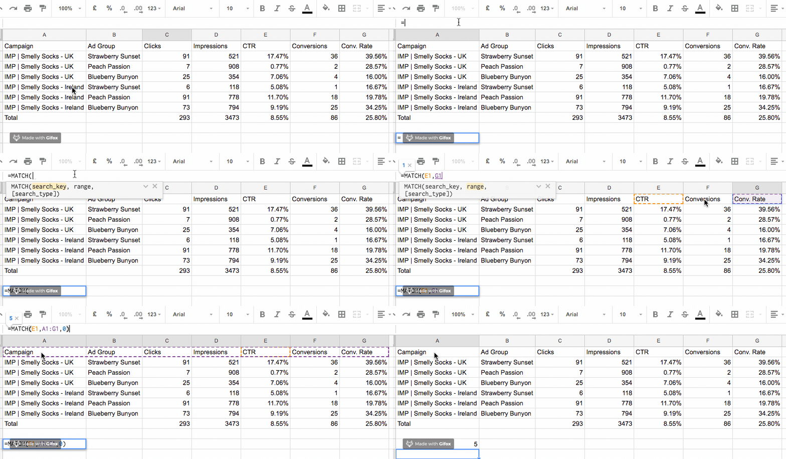
More importantly, if I rearrange my columns, delete a column or insert a column, providing one of the cells in the range I’ve selected says “CTR”, this MATCH function will tell you where it is.
It works in the exact same way for rows too. Want to know which row is the Total row? Piece of cake.
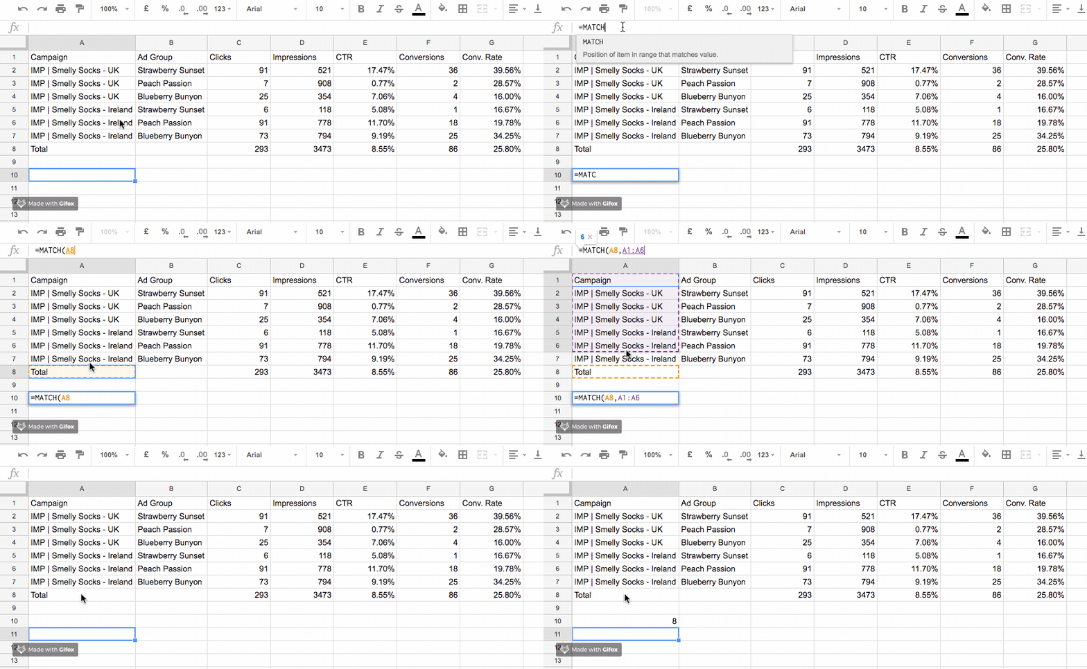
Got a really big spreadsheet or can’t be bothered to scroll? Just type the search key instead.

As you might have guessed, this is a game changer when combined with INDEX and an even bigger game changer when used for PPC.
How to use INDEX MATCH for PPC campaigns
You can use INDEX MATCH everywhere you’d usually use VLOOKUP.
Just this week, I’ve used it to create a German Google Shopping feed by matching product IDs up to their titles, categories and descriptions. I don’t even speak German, but because INDEX MATCH matches things up exactly, I don’t have to.
Let’s go back to Smelly Socks again to see how to combine INDEX and MATCH.

I want to look up the total number of conversions across all campaigns.
First, I use INDEX to select the table, writing 1 in both row and column as a placeholder.

This gives the value of the cell in the top lefthand corner of the table – A1 in this case. Now it’s time to replace each of those 1’s with a MATCH function. Since the first 1 corresponds to the row, I’ll use this one to create a MATCH function that selects the row containing the total.

Just in case you weren’t convinced, the MATCH function has (correctly) selected row 8.

Now it’s time for the column MATCH. Just like that, MATCH has correctly selected column 6.

Hit Enter and what do I get?

Boom: 86!
Even if I add, move or delete a row or a column (except the one that 86 is in!), I’ll always be given the right answer. THINK OF THE POSSIBILITIES.
Dynamic lookups with INDEX MATCH
Here’s just one of the possibilities that you might not have considered. Remember that I typed “Conversions” in the function? I don’t have to. Instead, I could just select the cell containing the value that I want to look up. No one says that cell has to be a cell in the look up range, only that the look up value itself has to be in the range.
That means that you can do cool things like this…
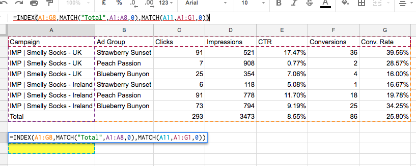
Now, instead of looking for “Conversions”, my column MATCH function will look for whatever is in A11, the cell that I’ve highlighted in yellow. That means that if I type in “Clicks”, I get the total for the clicks column.

You guessed it – you can do the same with the rows too! Imagine typing in the Campaign or Ad Group name and instantly being presented with all of the metrics that you want.
See? You’ve forgotten about VLOOKUP already.
Try dynamic lookups for yourself
I’ve made a little demo for you to try out the dynamic lookups for yourself.
Type one of the metrics in the top row (e.g. “Clicks”, “Conversions”, “CTR”) into the yellow cell and see what value the sheet gives you:
INDEX MATCH Dynamic Lookup Demo
Solemnly swear you’ll never use VLOOKUP ever again
It’s buggy, it breaks, it’s awkward. Please – just turn your back on VLOOKUP and don’t look back. You need a clean break. If VLOOKUP texts you after a couple of days saying that it can change, ignore it. You deserve better.
At Impression, we use a combination or technology and creativity to get the most out of our PPC campaigns. With so much information available to us, a VLOOKUP simply isn’t going to cut it.
In the constantly changing and data-driven world of PPC, we know that what you need is something future-proof, accurate and dynamic.
What you need is INDEX MATCH.
