Google Sheets is an amazingly powerful tool, free for all SEOs, that so many don’t use to its full potential due to lack of experience or knowledge. This blog shows 5 ways that certain formula, when implemented properly, will simplify the way you work, saving valuable time that could be better spent on SEO work.
Advanced Formula Examples to Help SEOs
1) VLOOKUP
=vlookup(string, range, index_key)
This is the absolute bread and butter for all SEOs in my opinion, so the first and most important advanced formula to master.
A VLOOKUP allows you to search a range using a string; you can then return matching values from a specific cell in said range.
Example

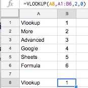
In the above example, I have used a VLOOKUP to pull data from column B (2) from the table that is specified by the range (A1:B6). This is deliberately simplified as an example.
More commonly, we can use a VLOOKUP to update data. For example, if I have keyword data from when I first started with a client and want to compare rankings 3 months later, I can add a column and VLOOKUP each keyword to get current and previous ranking position.
Note: As long as you specify the number, any column can be used to pull data (i.e. E= 5), as long as said column is in the range.
Additional uses
- Checking values against another data set to check for duplicates across two or more lists.
- Matching prospects to contact details in a master database.
2) IMPORTXML
=importxml(url, xpath_query)
This formula lets you import data (using an XPath query) without ever having to leave Google Sheets.
Useful XPaths
- Title: “//title”
- Meta description: “//meta[@name=‘description’]/@content”
- H1: “//h1”
- All links on a page: “//@href”
There are so many more XPaths and different types of information that you can pull in with Sheets. Play around and get used to this formula as it will definitely come in handy.
Example

This example shows a common SEO task made simpler. With a list of URLs in column A and the correct XPath implementation for IMPORTXML, current metadata can be pulled in and used as a reference for your optimisation. Additionally, the length can easily be measured using the LEN formula, see here for more details.
Yes, this data can be found from crawling sites such as Screaming Frog and Seomator, but the beauty of using IMPORTXML is that once this sheet is set up the current metadata will be pulled in. So rather than having to recrawl and check again, just refreshing the Google Sheet will give you up to date information.
3) OR, ISNUMBER, SEARCH & IF
=or(isnumber(search(term, string)))
This combination of formulae lets you identify terms which are incredibly useful for categorisation.
Breakdown
This formula combines 3 individual functions to give the desired output, broken down this is what each does:
- OR = Test multiple conditions with TRUE or FALSE output.
- ISNUMBER = Test to check if a value is a number returning TRUE or FALSE.
- SEARCH = This function returns the location of a substring in a string. The search is not case-sensitive.
An example of this in practice would be if you have an extensive list of target keywords that you want to attribute to a specific category or product page on your site for better targeting and reduce cannibalisation.
If your site sold women’s clothes, for instance, then a column could represent the Dress Page, and the formula in that column could search the list of keywords for related terms such as “dress, bodycon, day, party, maxi, midi, mini, swing, and summer”.
Example

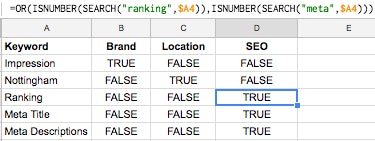
As many as 200+ terms can be searched in one formula thanks to the OR function, the formula just needs to be repeated for each term.
Finally to take the categorisation one step further, combining multiple IF formula can be used to create a category column. For further explanation of IF formula read the Top 12 Formulas for Beginners.
Example

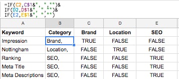
The above screenshot shows this at work. Column B checks if there are any TRUE statements and if so returns the title for that column.
Notes
The way this formula is set up means that if a keyword was matched by multiple searches (i.e. TRUE appeared for Brand and Location then this would appear in the category column as Brand, Location) all applicable labels would be listed.
In the above IF formula the ‘$’ is used “C$1”. The use of the $ enables ‘relative’ cell references, this symbol ‘anchors’ a column, row or both.
To anchor the cell reference I could place $ before both the column and row reference (e.g. +$A$1). No matter where this formula was copied on a Google Sheet it would always read +$A$1.
Additional uses
Checking through contact details of potential targets for remarketing or outreach, to check for any fake emails.
4) SQL QUERY
=query(range, sql_query)
Basically, this is a bigger, badder VLOOKUP that lets you query data using Structured Query Language (SQL). It gives the option to put multiple conditions in place when retrieving data as well as going into great detail.
The example I like to give when trying to explain the potential of a QUERY formula is compiling a backlink profile of a client’s 5 major competitors that you want to compare.
Exporting individual backlink profiles from Ahrefs or a similar tool you are likely to have 1,000+, if not 10,000+, backlinks to check through – some useless, the majority not.
This is where QUERY can come in and save a lot of time, using a formula such as:
=QUERY(‘Client Backlink Profile’!A:R,”select E where M contains ‘Dofollow’ and N contains ‘Active’ and D >50″,1)
When this formula is used on a new sheet it will produce a new list of your specified column from the master sheet. A screenshot, therefore, won’t particularly help to explain.
Breakdown
- In the above example formula, the range is as used in many formula such as VLOOKUP (‘Client Backlink Profile’!A:R).
- Specify the column you want to be listed in the new list produced; in this example column E is the referring page (“select E…”).
- Set the conditions that have to be met to be pulled into the new list. For instance, ‘M’ in the Link Type, and we only want to see followed links (where M contains ‘Dofollow’).
- Additional conditions can be added in conjunction (and).
- Filter out redirected, dropped, removed links by specifying that Backlink Status column ‘N’ has to contain ‘Active’ (N contains ‘Active’).
- Filter all referring pages where Domain Rating ‘D’ isn’t over 50 ‘>50’ (and D >50″).
- Finally specify how many header rows are used at the top of the range, usually this is just 1 (1).
Additional uses
- Create granular client-facing documents that pull in data from a master sheet
- With the ability to IMPORTRANGE to a QUERY it enables queries from other sheets
5) SCRIPTS
In Google Sheets, Tools has a Script Editor. Although not a formula, scripts offer powerful opportunities when understood and used properly. Moreover, on the uncommon occasions that formulas can’t solve the problem you have, scripts can come to the rescue.
The Script Editor costs nothing to install and allows you to do new and exciting things with Google Sheets, Docs and Forms. Google Apps Scripts provides a JavaScript cloud scripting language that provides easy ways to automate tasks across Google products and third party services and build web applications. Any scripts you input will run on Google’s servers.
Some of Google Apps Script capabilities include writing custom functions for Google Sheets and implementing custom menus, dialogs and sidebars, as well as publishing web apps that interact with Analytics, Calendar, Drive, Gmail, Maps and even with third parties using APIs.
Here at Impression the use of scripts came in very hand recently. An ecommerce client had thousands of duplicate meta titles and descriptions. Rather than going through the 2,500+ duplicate page titles one by one, IMPORTXML was used to pull in the H1 and H2 from each page.
The idea was that the H1 (Product), the H2 (Product Brand) and the ecommerce brand could be combined to give a unique and valuable title for each page.
Unfortunately for this site the H1 & H2 data weren’t being pulled through with IMPORTXML. If this is the case there could be a couple of reasons: either the site XML is not valid, in which case it can’t be recognised, or, if specific elements are dynamically created using Javascript, these elements may not be generated for IMPORTXML to scrape.
Here are a few core lines of the script, which are required to generate Title Tags from a html page:
var html = UrlFetchApp.fetch(url).getContentText();
The above line returns the html from a given URL.
var Brand = html.substring(html.lastIndexOf('<h2 itemprop="brand"><a href="">'),html.lastIndexOf('</a></h2>'));
The above line extracts the Brand term, which in this instance is within the H2 tag.The above line can be completed multiple times to extract various elements, such as product name and category. We can then use these to build the new Title Tag.
range.setValue(Product.trim() + " " + Category.trim() + " from " + Brand.trim() + " | Client Name");
The above line builds the tag using the product, category and brand, which is completed by adding our client’s brand at the end.


